Statistics and other links and thoughts, September-Mid October 2022

Here are some statistical and other links.

The previous linkpost in this blog was in August, so I have achieved a streak of 2! Or almost 2, as it is already October 13. Let’s call it two positive observations in the series of 2.41 months. Laplace’s rule of succession would suggest that we have a probability

\frac{2+1}{2.41+2} = \frac{3}{4.41} = 68.027%

of observing the next link post in the next month. Not too shabby, but not very trustworthy either. Which describes my feelings about continuing blogging this time around (I think I have had three hiatuses of various length, and WP statistic suggest about 3 readers, who may very well be bots). BTW, Laplace’s rule was the first link. ;)

Predictions

Suggestions of better scoring rules (for collaborative forecasting).

Comments: Sounds very neat, and much better than Keynesian Beauty Contest (for explanation in the prediction market context see eg this ACX post). I fear the suggested oracle method is susceptible to bad actors as oracles, though, in a way a regular prediction market ideally should not be. Though I feel any prediction market should totally not use money at all. Reputation-based mechanisms maybe could be salvaged?

Folk “theorem” 1: If a prediction market gives reward X for correct prediction, but if you as know there are benefits Y to be realized from influencing prediction market making everyone to believe in a biased prediction, and Y > X (and if you are homo economicus), you should try to influence the prediction markets.

Folk “theorem” 2: However, consider that the typical example for realizing such benefits Y would be something not unlike stock market trading or options or w/e. Comparisons to insider trading are easy. ANYWAY, making a trade that yields Y profit is possible because the other trader(s) (patsies) with bad information agree to it, thus they a trade at loss (compared to not making the trade if they had had non-manipulated information provided by prediction markets).

Analogues can be drawn to politics, elections, warfare, etc; the issue is not strictly limited to financial instruments.

The point being, would-be patsies are aware of point 1 and have an incentive not to be patsies. They also totally should spend money in prediction markets to over-correct any probabilistic bad actors.

And finally we have a folk … uh, let say it is a folk conjecture: Doesn’t all the above suggest that any liquid, publicly known prediction market coupled to the other global economy will eventually subsume all of the markets (previously known as the real world), as everyone tries to extract profit by either trading their information or misleading the prediction markets against their better information if it worth more in the non-prediction markets … ?

VATT

(Finnish state-funded) Institute for Economic Research VATT tweeted many interesting papers about economics of housing during their VATT-päivä seminar. In English, in Finnish

Then I found that VATT + Tilastokeskus + Helsinki GSE have an interesting initiative for producing fast-paced research / policy briefs called Datahuone. I don’t know if it is going to be different than research institutes / think tanks usually do, but finding good think tanks in Finland is difficult, and special bonus if they manage to produce topical outputs.

Long-term effects of Chinese revolution

Okay, somehow my October was very economics-heavy. Here is The Economist and social capital of grand-children of pre-revolutionary Chinese elite. I quote two nice graphical visualisations that explain the main point

Source: The Economist, Jun 9th 2022, The grandchildren of China’s pre-revolutionary elite are unusually rich. Their original source was, “Persistence despite revolutions”, by A. Alesina, M. Seror, D. Yang, Y. You & W. Zeng, working paper, 2022

(How to not) pseudocriticize

(We are now approaching genuine statistical content!)

Stuart Ritchie in his Substack: Pseudocritics, and how not to be one

Summary: People love looking at scatterplots and arguing them supporting / not supporting some particular hypothesis (I myself do this a lot!) One should bear in mind that quantitative, numerical statistics is most needed in judging random-looking scatterplot clouds. After all, quantitative result says how random they are (under some assumptions, naturally), and one would not ask if it wasn’t in dispute.

Latent factor models

S. E. Heaps, http://arxiv.org/abs/2208.07831 “Structured prior distributions for the covariance matrix in latent factor models” 16 Aug 2022

Comments: I saw a comment somewhere (unfortunately didn’t write down where) that Heaps has managed to derive a Bayesian latent factor model with prior + sampler that is quite useful. Examples include using phylogenetic-tree prior for bird observation data factorization.

Fitting such models naively can be a little painful in my experience. I hope I won’t forget about this, that why I am writing it down here.

Improving your statistical inferences

Lakens has published now (free, CC-BY-NC-SA) online textbook called Improving your statistical inferences. The parts I have read are not very complicated or technical if you already possess familiarity with statistics, but that just makes it then a not-too-heavy reading: graphics look intuitive and principles well-explained, so chances are, it could improve my statistical inferences!

R packages

targets looks like a cool way to manage pipeline dependency targets.

box appears to provide a handy way to avoid source() function spaghetti without moving to R package development. Downside: one needs to learn a quite different framework.

That’s all for this time.

Reading How to Measure Anything, interlude 2

(Summary in Finnish: Lukupiiri on päättynyt jo jokin aika sitten! Puhtaaksikirjoitetut oppimispäiväkirjamerkinnät ovat olleet tauolla ja palaavat joskus, toivottavasti pian.)

Context: This is a quick interlude note in a series of learning diary notes, where I track my thoughts, comments, and (hopefully) learning process while reading How to Measure Anything by D. W. Hubbard together with some friends in a book club setting. Previous parts in the series: vol.0, vol.1., vol. 2, interlude 1. All installments in the series can be identified by tag “Measure Anything” series on this blog.


Interim report

Howdy! This interlude note serves as a brief status report concerning the learning diary entries for How to Measure Anything. Until the rest of the entries are online, this post also explains why there are no (yet) further installments.

As everyone of three or so of you who were determined to push through to the end of the How to Measure book already knows, the book club concluded some two months ago. I have bunch of notes and blog post skeletons from the book club meetings, but after the first couple of posts, I developed a syndrome characterized by debilitating symptom of “I want to write these blog notes in good English” and consequently updates are quite sluggish because (I now try to proof-read and copyedit the posts for bad grammar). Also, I managed to get full-time employment, so I suddenly have much less free time and energy for hobby activities (especially those that resemble real work).

The fact that I also bought Europa Universalis IV from Steam sale have nothing to do with me having less hours for blog-writing, no whatsoever (a lie).

Reading How to Measure Anything, interlude 1: Bayesian and frequentist inference

(Summary in Finnish: Oppimispäiväkirjamerkinnät jatkuvat hitaasti. Tässä lyhyt lukusuosituslinkki Bayes-päättelystä.)

Context: This is a quick interlude note in a series of learning diary notes, where I track my thoughts, comments, and (hopefully) learning process while reading How to Measure Anything by D. W. Hubbard together with some friends in a book club setting. Previous parts in the series: vol.0, vol.1., vol. 2. All installments in the series can be identified by tag “Measure Anything” series on this blog.


Introduction

Despite the radio silence, the reading club has been marching on steadily but quite slowly. I have work in progress drafts for notes vol. 3, 4 and 5! Unfortunately other life has intervened with finishing the drafts, so the next installments of reading log entries will come up online here on the blog … sometime later.

However, as the book discusses in several places “Bayesian probability”, I thought it would be prudent to share some links to articles that actually explain what it means. (As I am a bit too busy to write a thorough lecture on myself, I will rather defer to experts.)

Without further ado, here are the links:

Difference between Bayesian and frequentist inference

Very shortly described: The frequentist inference is concerned with interpretation of probability, where probability is understood as property of repeated, independent events (“frequency”). Bayesian inference builds on Bayesian interpretation of probability, where “probability” is taken to be a thing that exists for anything, interpreted as quantification of knowledge about many different things. This kind of interpretation makes it possible to sensibly interpret and use Bayes theorem for inference about various random variables.

This is a succinct definition by a person who has had some years of experience working on this stuff, and it might not much sense if you are not already familiar with it.

While looking for something else entirely, I noticed this five-part series of blog posts by Jake VanderPlas. It illustrates the above brief statement in more detail. I recommend the first part (which I have actually read), as it is quite practical example. However, as a word of warning, the author is an astronomer, so for them “practical” includes use of some mathematical notation and calculations.

For a discussion about implications of these concepts, here is a nice pdf of class notes from Orloff and Bloom, MIT.

This Stat.StackExchange answer by Keith Winstein is great explanation how the difference works out between frequentist confidence intervals and Bayesian credible intervals. It involves chocolate chip cookie jars!

Bio-statistician Frank Harrell has a blog post titled My Journey From Frequentist to Bayesian Statistics. It also collects further links at the end.

Use of Bayesian statistics is not always very Bayesian in practice

Have you read all of the above?

Good! Here are some thoughts related to the real-life applications of Bayesian inference.

In addition to all of the above, there is a certain internet crowd who likes to use words like “prior”, “Bayesian belief” and “Bayesian update” for many things because “rational agents are Bayesians”. I do not say it is not useful to have such a concept and thus word for inductive reasoning (or, as one may say, “Bayesian update”): if you have a prior state of belief, and then obtain some new information, and if one can quantify the prior and the likelihood of data with with parametric distributions or probabilistic statements, the Bayes’ theorem will tell you what is the mathematically correct probabilistic state of belief (the posterior). (And if you skip the step of quantifying the numbers, one could still argue the procedure of obtaining the posterior belief should look like application of Bayes’ Theorem if one were to put numbers on it, which maybe gives some intuition about reconciling ones beliefs about some matter with new evidence.)

However, more one works with explicit, quantitative Bayesian statistical models (like presented in the VanderPlas blog series) it starts to sound a bit weird to talk about “updating ones belief” without making calculations with any models or probabilities.

It gets even more weird when practicing statisticians (who write authoritative textbooks on Bayesian data analysis) explain that actually, in real life, the way they do Bayesian statistics does not resemble an inductive series of Bayesian belief updates (pdf):

A substantial school in the philosophy of science identifies Bayesian inference with inductive inference and even rationality as such, and seems to be strengthened by the rise and practical success of Bayesian statistics. We argue that the most successful forms of Bayesian statistics do not actually support that particular philosophy but rather accord much better with sophisticated forms of hypothetico‐deductivism. We examine the actual role played by prior distributions in Bayesian models, and the crucial aspects of model checking and model revision, which fall outside the scope of Bayesian confirmation theory. We draw on the literature on the consistency of Bayesian updating and also on our experience of applied work in social science. Clarity about these matters should benefit not just philosophy of science, but also statistical practice. At best, the inductivist view has encouraged researchers to fit and compare models without checking them; at worst, theorists have actively discouraged practitioners from performing model checking because it does not fit into their framework.

Gelman and Shalizi, “Philosophy and the Practice of Bayesian Statistics.” British Journal of Mathematical and Statistical Psychology 66, no. 1 (2013): 8–38. https://doi.org/10.1111/j.2044-8317.2011.02037.x.

If you feel like reading 30 page of philosophy of statistics, read the whole article. The way I read it, looking at the whole of knowledge-making produce of successful practical statistics, which includes the part where (1) one formulates the Bayesian model and priors about some phenomenon, (2) fits the model to data and obtains the posterior inferences with math and algorithms, and (3) then checks if it really works with various other methods, only (2) is really about making Bayesian updates. In combination with parts (1) and (3), the whole procedure is more hypothetico-deductive than inductive, and model checks that have some affinity with Popperian falsifications.

If you want to read more about this kind ” statistician’s way of doing” Bayesian inference, you can read a more recent article “Bayesian Workflow” by Gelman et al. 2020 (arxiv) which presents a comprehensive and quite technical 77-page step by step tutorial into it, or less comprehensive but also quite mathematical essay by Michael Betancourt (2020), “Towards A Principled Bayesian Workflow” (html).

Reading How to Measure Anything, vol. 2

(Summary in Finnish: Oppimispäiväkirjamerkinnät jatkuvat, hitaasti mutta kumminkin. Aiheena luvut 3 ja 4; luvusta 3 löysin paljon sanottavaa kun aloin kirjoittamaan.)

Context: This is a part in a series of reading / study diary notes where I track my thoughts, comments, and (hopefully) learning process while I am reading How to Measure Anything by D. W. Hubbard together with some friends in a book club like setting. Links to previous blog entries: vol. 0 (introduction); vol. 1. All installments in the series can be identified by tag “Measure Anything” series on this blog.


This part of the series is quite behind the schedule of the book club (we have already discussed Chapter 7 and will talk about 8 & 9 this week). The reason for the lateness of the current installment is that I felt inspired to say quite much about Chapter 3 when I reviewed my notes some time after the book club meet.

Summary of lessons from Chapters 3 & 4

In Chapter 3, Hubbard presents more detailed discussion of concept of “what is measurement”. . In the following chapter, we start our journey into studying the concepts how to measure something (hopefully, anything) following author’s advice by talking what is a practical measurement problem.

On Chapter 4, which discusses framing a good measurement problem, I have much less to say.

Onto it!

Measurement as approximation

Hubbard starts Chapter 3 with a quote from Bertrand Russell:

Although this may seem a paradox, all exact science is based on the idea of approximation. If a man tells you he knows a thing exactly, then you can be safe in inferring that you are speaking to an inexact man.

—Bertrand Russell (1873–1970)

…while Hubbard has much more to say, the quote summaries the point I’d consider my most important take-away from Chapter 3. The exact measurements are rare-to-impossible; modern science and engineering is concerned with approximations or (even better) quantified tolerances.

The reason I consider this personally the most important lesson to me is that I was both surprised yet I should have know this: for my master’s thesis, I studied a set of tomographic reconstruction algorithms for X-ray computed tomography of pipe section welds for industrial applications. While the particular application and set of algorithms I experimented with were relatively novel, the relevant technology in general is example of established field of science and engineer: in medical applications, CT scans are something people trust. Yet every such device has to deal various sources of noise and measurement imprecision. At the very best, I can quantify the amount of error in ones measurements in a way I can trust. This does not preclude improving the method so that the amount of error gets small enough for the desired purpose. However, to convince myself and others that the amount of error is bounded, I need some kind of proof of it.

Likewise, one of the important part to consider when applying any practical, numerical algorithm to solve any mathematical problem is the formal quantification of amount of error in the numerical solution.

A digression to demonstrate this. Consider a classic dynamic system (Wikipedia) that models a closed ecosystem with one predator and one prey species population, where the predator (say, lynx) feeds on the prey (say, rabbits). Let us assume the rate of change of size of predator population at any given moment depends on availability of the prey and similarly for the prey population. This results in boom bust cycles for both (plot). Given the mathematical equations for this kind of dynamical system, the most classic and easiest method to “draw” this kind of a plot for a described dynamic system is to calculate the evolution of the system at each individual time point, step by step with step length h: if we know number of rabbits and lynx at time point $t$ and the how their number depend on each other, compute their number at time point $t + h$. This process is known as Euler method. While easy to understand, the other important thing to know about Euler method is that it has a provable error proportional to h^2 on each individual step, which can be noticeably improved with better algorithms. Such considerations are bread and butter of any serious application in numerical methods. The lesson: mathematics is often considered a field of precise answers (and not unjustly so!) Nevertheless, when one enters field of one numerical solutions, mathematics becomes about being quantifiably imprecise. [/end of digression]

So, considering all of the intuition into measurement and error above, I am quite appreciative to Hubbard’s central claim of the chapter 3: obtaining approximations that are good enough is the useful standard of measurement is a good standard definition for measurement. Thus it the other central claim is also plausible, namely, reducing ones uncertainty is also a measurement in more fuzzy domains – or domains incorrectly viewed as fuzzy and intangible.

Rest of Chapter 3

Other points worth noting from Chapter 3 include some discussion into how to define the thing being measured, about methods for measuring things and some common objections, such as when it worth the cost of measurement to measure things.

First, the object of measurement. Hubbard argues (quite convincingly) that if anything is considered important, the qualities that make it important have noticeable effects on the wider world. Consequently, if these effects are noticeable, they also can measured rigorously. This is demonstrated by several more or less persuasive examples from author’s career in consulting (which I see no point in repeating here, read the book yourself).

My only reservation is that while the chain of reasoning is quite valid in abstract, for some qualities the useful practical measurement may be prohibitively difficult (expensive), but maybe this will be discussed in more detail in a later chapter concerning value of information.

Secondly, methods of measurement. Concerning the methods, the book actually makes two distinct points. The first one is that there are many established statistical procedures for measuring various quantities about unknown quantities of any population. The second point is a couple of simple rules that illustrate how small amounts of good information tell a lot more than nothing. Consequently, when one does not know anything, almost any effort at knowing more is very useful. This is surprising, and I am half convinced

This is demonstrated by two statistical “rule of thumb” theorems that are quite surprising (or maybe not) and I think are worthwhile paraphrasing here in more detail:

The Rule of Five. There is a 93.75% chance that the median of a population is between the smallest and largest values in any random sample of five from that population.

Remember, the median of the population is the point that separates that mass of the population distribution in half. If you feel inclined, working out the proof the statement is quite trivial from that fact, and assuming one takes five independent samples. At first the statement sounds quite surprising, almost magical: five samples from a population is not a lot. However, if one has a very wide or otherwise not nice underlying distribution, the minimum and maximum of the sample of five is quite likely to cover a wide range.

The Single Sample Majority Rule (or, The Urn of Mystery Rule). (Rephrased.) Assume a population with a binary quality. such as, an urn that contains balls that can be of two different colors. If the proportion p \in [0, 1] between different colors is unknown and one considers all proportions between equally likely a priori. Under these assumptions, there is a 75% chance that a single random sample is from the majority of the population.

Again, the proof is not difficult. (Hint: Start by noting equal probability for all p or p \sim U(0,1). Suppose one has drawn a ball of one color. Consider all possible proportions p from 0 to 1 for that color. (Alternatively, consider all possible urns.) Given the color of the drawn ball, the probability that the ball is from the majority corresponds to how many cases of drawing a ball with the same color …? Draw a figure.)

However, I said I am halfly convinced. The argument is two-pronged: Yes, both the Rule of Five and the Urn of Mystery Rule sound surprising. Approximate 94% chance that the median of a population is withing five independent samples from it sounds large, and is useful to know, but as I said, with large distributions that range can be surprisingly large. Likewise, in the Urn Rule, 75% is a lot, but so is 25%, and it is based on assuming an uniform uncertainty about the true proportion. Uniform distribution is a reasonable choice in that it is a maximum entropy distribution between 0 and 1, or in layman’s terms, it conveys maximum uncertainty about a quantity given the upper and lower bounds for quantity’s range. However, sometimes one knows more than nothing, which has noticeable effects.

On the other hand, if one does not really nothing, the Urn of Mystery Rule still applies only to observation about a single binary quality. Why this is important caveat?

Example. Consider the population of students at one particular university, and let us assume you meet one of them (single random sample). Choose one quality of student, for example, whether their GPA is high or low (defined as GPA \geq 3 on scale 1 to 5, for instance) and call the groups “high-GPA” and “low-GPA”. Without any other knowledge about proportion of “high-GPA” to “low-GPA” students, there is a 75% chance that majority of the students in this particular university belong to same GPA group as this student. However, this breaks down if you know that university’s grading policy is not independent but grade distribution is normalized to follow some fixed distribution. Even if they don’t (maybe all professors maintain their own idiosyncratic grading policies that are set in stone), this is only one quality. Choose some other binary quality, for example, whether they are tall or short (according to some arbitrary threshold). Again, if you don’t know anything else (like, underlying height distribution in the country), assume equal probability for all proportions and meet a student who is tall (or short), there is a 75% chance that majority of the students are also tall (or short). Same for other accidental qualities: Whether one of their parents also went to university, whether they like the color blue, whether they know how to program in LISP, etc.

However, if you don’t have any reason to believe that these qualities are correlated, and the student you meet is tall LISP programmer who wears clothes with lots of color blue and has high GPA and highly educated parents, the probability that the majority of the student population is likewise in all these qualities is $0.75 \cdot 0.75 \cdot 0.75 \cdot 0.75 \cdot 0.75 \approx 0.237$, which is (i) much smaller number than 0.75 and becomes more smaller more qualities about the person feel salient to you and also (ii) unrealistic, in the sense than one probably has better than total uncertainty about things like popularity of LISP. Moreover, if you consider qualities that are not easily thought about as a binary (e.g. hair color), the calculation becomes different. [/end of example]

Nevertheless, I can not find myself disagreeing with the counterpoint of counterpoint: If you know nothing of the population before taking the five samples, even a very wide range for the median is more than nothing. Same for drawing the first sample from totally unknown population. But one should be aware of hos strong the words of “nothing” and “unknown” are.

edit.And additionally, these considerations illustrate that realizing any small amount of information one has about the subject topic may greatly influence these kind of simple calculations!

When it is worth the costs to measure things?

The question of when it is worth the effort and the inflicted costs to measure something sounds like the final important part of Chapter 3, but in it is not answered in depth. Hubbard’s thesis is that measurement is valuable when there is high cost of being wrong tied to large amounts of uncertainty. There are several examples of common objections (“economic arguments against measurement”) and counterarguments, but I think the basic gist is this: If one wants to argue that measuring something is too difficult or too expensive, one should consider also the difficulties and costs entailed in the case the uncertain risk is realized in an unfavorably way.

(If there is a knowledge that there is no risk or it is acceptable, one already has enough “measurement”. Sounds a bit circular, but circular rephrasing makes the concept easier to appreciate..)

Sounds good in principle, but how to do such comparison in real life? The disappointing answer is, the topic is not much discussed here, but as I have the benefit of progressing some chapters forward in the book, the answer is that a more detailed answer to the question will be explored in later chapters.

Goodhart’s law

I was also quite eager to see when and what the author in favor of “Measuring Anything” would address the Goodhart’s law, which (if you are not familiar with it already) is commonly stated in following words:

When a measure becomes a target, it ceases to be a good measure.

Dame Marilyn Strathern, apparently

For some reason, it is dealt with as one of the “economic arguments” in this chapter. The author acknowledges the dangers, but argues that making measurements and creating incentive structures (that involve measurements) are two different things.

…which, as far as counterarguments go, does not impress me too much. I would argue that the important thing to understand of the Goodhart’s law is this: Making measurements that influence decisions that affect people is a reason for the affected people to adapt their behavior. Sometimes or often some kind of change is wanted, but people can surprise. If the method of measurement is public knowledge, then it becomes (of course) one of the easiest things to adapt to.

The reason why situation is problematic for audience of this book may become more obvious if it is written as an adversarial measurement scenario. Let us imagine party A, having read “How to Measure Anything”, who wants to makes measurements M of some features of intangible target T to make decision which involves interests of another party B. If also the party B has read the book “How to Measure Anything”, they would probably like to measure how to best affect the decisions of part A! If party B can affect both T and M, then they would naturally want to evaluate which one they should work on. (Usually the problem is that M, being specified, is more legible and thus easier to influence than the intangible target that A is really interested about).

I am not super familiar with the relevant game theory and economics, but it seems there would be quite much interesting things to discuss about strategies that arise in this kind of scenarios. Unfortunately, it seems it is an interesting topic for some other book.

Consequently, why continue reading the book? My personal take is that it is fine to follow the way of this book and make measurements without such strategic considerations either if (a) the scenario is not adversarial or (b) if there is an adversarial party involved, they are not measuring your measurements. (Someone might say something about countermeasures.) It feels intuitive to argue that either the measurement is one-off and secret.

Lessons from Chapter 4

Chapter 4 deals with the question how to measure with lots of practical advice and examples, which sound very sensible.

The basic point is quite simple: The problems that appear difficult to made quantifiable can become much easier if one carefully reiterates why the problem is important. Usually this is because there are decisions involved. The first step in Hubbard’s five-step workflow to do this iteration is “defining the decision”: Define what are the stakes and what are the alternatives, which leads to neatly to step 2, determining what you already know about both.

It sounds very simple, but also quite useful. As I said, the book fleshes this out in more detail (so if you are not convinced, maybe read the examples in the book by yourself), but the above is the best summary I think I can make. Techniques such as Fermi decomposition can help, but I feel lots of advice is also quite context dependent.

Measuring relative vs absolute quantities

One point that is mentioned in passing but worth I thought highlighting: when one frames the measurement problem as problem of choosing between two alternatives, both associated with one numeric quantity each, it is not necessary to established absolute magnitude for either. It often suffices to establish the relation between them. Magnitudes matter only to the extent that one must make sure the two quantities are comparable.

Thinking about it, it makes sense: with compositional data, one can say quite many things about relative importance of two quantities by fixing only their relative size. In some applications, fixing the magnitude of the quantities requires.

(Remember my example about dynamical system of rabbits and lynxes? One does not need to count all the rabbits and lynxes in the ecosystem, usually one tries to estimate them with some kind of observational sampling.)

Other points (from the book club discussion)

My discussion notes are not as extensive, and I am writing this nearly two weeks after the discussion. As far the notes go, we apparently mostly talked the main contents of the chapters at hand, reviewed above.

In addition to above,

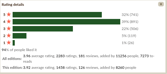
  • we got a reading recommendation: Moral Mazes by Robert Jackall (Wikipedia, GoodReads). (Correction:2021-02-24 The recommendation was for a blog that discusses Jackall’s book.)
  • While I did not think it very interesting, book discusses terminology related to Knightian uncertainty. (Hubbard defines “uncertainty” as a lack of certainty and something you can put a number on, and “risk” as uncertainty involving a loss. Knightian meanings for “uncertainty” and “risk” are different.) We talked about about the wider concept of not-quantifiable uncertainty as form of “unknown unknown” as compared to known unknowns.
    • See also https://en.wikipedia.org/wiki/Ellsberg_paradox.
    • Example of “unknown unknown”: Members of the book club anticipated many various distractions and failure modes for a reading circle. For example, it was not a total surprise that one member was too busy to attend. However, all present were very surprised when we realized that some of us had been using different editions of the book with much difference in the content!
  • Related to above, some people have found some use from Cynefin framework.
  • In general, there was some amount of agreement that thus far the book as been more conceptual than technical, and we have been familiar with some of the ideas before. (E.g. via Effective Altruism.)

Conclusion

The chapter 3 started with a blast, by pointing out how measurements can be useful despite them always involving some kind approximation and error. In my comments, I tried to highlight how quantifying the amount of approximation alone can be important! Chapter 3 also talked about various methods of measurement, where I found the two statistical rules (the Rule of Five and the Urn of Mystery) especially salient and worth elaborating. Other important topics included Goodhart’s law (Ch 3) and importance of stating the good measurement problems by identifying the decisions they are about (Ch 4).

I have no further conclusion to write! In our book club, we have already also talked about chapters 5,6,7, which I will write about in the next installment in the blog series. (Hopefully the next post will be public quite soon-ish.)

Reading How to Measure Anything, vol 1

(Summary in Finnish: Oppimispäiväkirjamerkinnät jatkuvat. Luku 2 oli paljon lyhyempi kuin kuvittelin (luen ekirjaa joka ei näytä sivunumeroita), joten suurimmaksi osaksi tässä kirjoituksessa keskityn lukupiirikeskustelun pohjalta nousseisiin havaintoihin ja ajatuksiin.)

Context: This is a second part in a series of reading / study diary notes, where I track my thoughts, comments, and (hopefully) learning process while I am reading How to Measure Anything by D. W. Hubbard together with some friends in a book club like setting. The first part in the series (vol.0) can be found here. All installments in the series can be identified by tag “Measure Anything” series on this blog. (Edit2021-02-24 : vol. 2.)


Summary of lessons from Chapters 1 & 2

Chapter 2 was much shorter than I anticipated! If you don’t recall, in Chapter 1 Hubbard outlines his basic thesis, which is (very briefly stated) that anything is measurable. Specifically, any and all quantities related to vague, often socially embedded stuff in business and government (“how much value we get from certain quality standards”, “how much value buying the product X to brings to us?”, “what are the effects of decision Y”) that are often thought impossible to measure. This can be done by applying correct, rigorous methods and enough effort into doing it. (Or that is the elevator speech for selling the book.)

In more detail (which I briefly touched in vol. 0), the primary purpose of measuring anything (in Hubbard’s words) is about reducing uncertainty about decisions. This can be done in many ways, starting from simple data acquisition and collecting them in Excel sheets, ending with quantitative models, and (Hubbard argues) this generally trumps mere intuition alone (because people tend to overvalue the soundness of their intuition). While perfect certainty is seldomly obtained, argument is reduced uncertainty from the measured data but also the act of thinking about what one can and should measure, helps making better decisions. Hubbard dubs the process presented in the later chapters of the book as “Applied Information Economics”, with following simple steps:

1. Define the decision.

2. Determine what you know now.

3. Compute the value of additional information. (If none, go to step 5.)

4. Measure where information value is high. (Return to steps 2 and 3 until further measurement is not needed.)

5. Make a decision and act on it. (Return to step 1 and repeat as each action creates new decisions.)

– How to Measure Anything, ch. 1.

However, the author grants that the audience may remain skeptical! So, in the chapter 2 of How to Measure Anything, we have some examples that illustrate how measurement solution may exist. The first two are examples with many are familiar, the third a bit less known.

First is Eratosthenes’ measurement of Earth’s circumference. The story and measurement themselves are quite well known, so instead of repeating it here let me link to Wikipedia’s explanation. (Did you know Eratosthenes was famous also for a prime number algorithm and was an acquaintance of Archimedes?) The second set of examples consists of a series of puzzles in the style made famous by Enrico Fermi, thus popularly known as Fermi problems. (How many piano tuners there are in Chicago?) The third example presents a school kid who set up a legit experiment to measure the effects claimed para-psychology-adjacent therapy for school science fair and consequently debunked it (with assistance James Randi; the details are bit long-winded to repeat here, but they don’t matter for the point being made).

The common property with all above-mentioned examples is that they demonstrate how measuring something is often possible with only minimal resources and thinking carefully what you already know. (Eratosthenes achieved remarkable accuracy with simple methods and measurements that were practical in his time. Fermi’s method for finding number of piano tuners does not involve any new measurements at all.) the science fair example is also similar in spirit: despite that the (claimed) phenomenon under investigation is supposed to be complex and mystical, is sometimes often enough to identify a core mechanism that would produce an easily understood measurable effect, which can be measured with simple methods (available to schoolgirl preparing a science fair presentation.

Points made during the discussion

So, what we though about it? I am not making an attempt to write a coherent nor all-inclusive recap, but present some of the more interesting ideas that came up. (Many of them are not mine! But I worded them from my notes in a way that I find interesting. Also I forgot to record who was saying what. I also have the benefit of writing everything here during the course of several days afterwards the discussion session.)

  • My previous point about it having a tone of stereotypical American “business self-help” was met with some agreement. However, in retrospect, maybe some other could say that this kind style is just being effective at conveying information to a certain kind of audience. And anyway, the quintessential self-help book, How to Win Friends and Influence People contains a lot of sound advice.
  • We talked how useful it is to have these kind of books that focus on the practical stuff. Many statistical textbooks remain difficult. It is also good to remember that while people like Galton, Pearson, Neyman, Spearman, Fisher and “Student”, who are usually best known as names for very abstract and theoretical, dry things in your statistic textbook, actually worked on many practical problems. (“Student”, that is, William Gosset used pen-name while publishing his paper on t-distribution because he worked at Guinness studying small samples and (presumably) Guinness did not want to their competitors know about the applications.)
  • Someone pointed out this: There may be at least one potential problem with applying the lessons from this book in practice, which is that sometimes the perceived inability to measure the “intangible” is a feature, not a bug. Many people and many organizations claim they have objectives, targets, values and whatnot that are written in official programs and defended in loudly spoken statements, but those targets are not what they are really trying to achieve. The act of claiming to have some particular objectives serve some other purpose. Giving the behavior a more benign interpretation, such publicly-stated objectives may be only a part of larger set of objectives that are left unsaid. A true, factual instance of greenwashing would be example of this phenomenon; in such scenario, an org that greenwashes their product would not want anyone making a truthful evaluation about their product’s environmental impact.
    • However, while I agree it is good to be aware of such things, I am not convinced how to usefully take such consideration into account while making decision when to engage in an analytical, quantitative decision-making procedure (like the one Hubbard presents). Afterwards, when I tried to come up with more examples of situations where organizations or individuals falsely pretend to be interested in either undervaluing or overvaluing something intangible, I concluded that collecting the information would be useful if you are in position to make a decision about the matter in the first place. Conversely, if you are a nobody in the hierarchy and can’t affect the $thing, it won’t make much difference if you find out how much value the purportedly intangible $thing has or makes, so maybe researching the matter is not very good way to use your time. (And maybe it is: if you know that the organization is allocating resources in sub-optimal way, and while you can’t affect it, it may be useful consider while making decision. Sell the stock? Vote for a different party? Relocate from the municipality? Brush up your CV?)
  • It seems that the book is going to take quite pro-“quantitative models” stance. We were interested in reading more how the book tackle’s the different kinds of uncertainty. The probabilistic models often present many ways to quantify uncertainty in the phenomena being modeled. (That is already what the classic P-value does: it states the numeric uncertainty of observing a particular set of data under some specific model.) But how to take into account — or even quantify — the uncertainty about your model being wrong? Some useful google search terms for learning about this more are aleatory and epistemic uncertainty. Many other forms of uncertainty have been defined, too.
    • While writing this write-up, I noticed that the author makes quite strong commitment while arguing how reducing uncertainty is beneficial and important. I started to wonder that such simple language masks quite many difficulties in what it means. See for example, bias-variance tradeoffs often discussed in machine learning textbooks. Suppose your uncertainty about true value of some parameter can be depicted as a normal distribution. Would you want to tighten your estimate by making the distribution less broad (smaller variance/s.d.)? What if it comes at a cost of your distribution being very tight and narrow but around a wrong (that is, biased) estimate, when previously you had more uncertainty mass covering also the true value? If you are making decisions based on the central parameter estimate and on it only, what matters is that the central moment of your uncertainty distribution is correctly positioned, not its s.d.
    • Also vaguely related to the above points, the book presents an example where some limited Fermi estimation is useful in determining whether to start up a particular kind of business in some region (whether there is enough customer base, and so). A counterpoint was raised: according to anecdotal stories (and maybe common sense building a successful start-up business seems to require something more than relatively simple calculation exercise with numbers. (Common sense, because many start-ups by persons who can make rational calculations fail and birth of new business empires are rare.) I am not sure what about to think about this objection. Maybe it is a case that easy-sounding examples look too easy because the truly valuable information necessary to build a successful company (or any other enterprise) is difficult to obtain and requires non-trivial insight, analysis, or luck. (But if it can’t be taught in a book, what is the point of reading a book?) I do not know. Let us continue anyway!

  • Related to the point about value of truthful information being related to your position or (in more generic terms) opportunity to use it, I found the subsequent discussion on power relationships in measurement particularly insightful. (In retrospect, this was probably a half-formed reinvention of ideas coming form Foucault. Sometime reinventing a wheel is still an useful exercise in learning the art of wheel-making?)
    • The argument raised was that introduction of formal way to measure something or anything, in practice usually in form of metric, is a form of wielding power. If you have an annoying productivity metric imposed on you, you are certainly not in control of the situation. People are often skeptical of metrics given by others, and often like to present objections related to what is measured and how the information is used.
      • The issue seem to disappear when you are making measurements for your own benefit. Example: Many people like the walk distance / step number counters nowadays common in phones and gamify their exercise routines. (Some other acquaintances of mine recently simply decided walk to Mordor.)
      • However, while I was in school, every winter the teacher handed out a photocopied piece of paper with ski-shaped progress bar, where every pupil was supposed to track how many km’s we skied during that winter. My parents put it on refrigerator, where my slow progress loomed over me menacingly. It was a very 00s Finland thing. I hated it.
      • I also think many people would view with suspicion if government required everyone to wear a walk meter and would put some metric targets where every citizen is required to walk to Mordor for national health benefit. Or your insurance company would require you to wear one to calculate premiums.
    • A bad metric may become a target and distract everybody from what really is going on and what was the phenomena supposed to be measured in the first place.
    • In a more adversarial setup, it may become a move to intentionally suffocate a rival organization by introducing wrong metrics, misleading metrics, or metrics that simply distract.
    • In my opinion, all this sounds like a very good reason to learn how to reason which metrics should or should not be applied, and how to make good measurements, and also present to reasoning convincingly to others.
  • As someone pointed out, all of this seems obviously related to principal-agent problems.
    • And also related to the benefits of free market based economies in contrast to central planning. In a country-sized unit, if there is a single authority who has the power to set the metrics for all industries, there are a country-sized amount of opportunities for them to fail in interesting ways. (Metrics becoming detached from things they are supposed to measure; people lower in the command chain misrepresenting the figures they report; mistakes in designing the metric and acting on them; the full difficulty of solving too large optimization problems to make the optimal decision…) Having smaller units where the decisions and the measurements they are based on are more close to each other and the underlying reality seems to way to both sidestep measurement problems and also bring the agency close to the level of individuals concerned.
  • Finally, (I think this idea was mine) precommitting into making a decision based on the results of some particular measurement procedure can be a powerful tactic, at least in two ways:
    • If you seriously consider the possibility that the decision is going either way based on the information you obtain, it highlights the need for good information. It should motivate one to set up the experiments, measurement methods, and other details very carefully, and encourage thinking about the problem. What exactly are you going to measure? (I believe Taleb would write about “having skin in the game”.)
    • It would also help to combat any internal psychological biases that otherwise could enter the decision-making procedure.
    • On the other hand, there is always a possibility that you simply made a mistake in the measurement process. I suppose that for that reason, measurements need some ultimate feedback from real life.

Other links:

Conclusion

As the reader may notice, the discussion points I recorded above are quite general, instead of addressing the content of Chapters 1 and 2 in a very detailed and immediate way. While I did not write everything we talked about in the meeting (only my reflections afterwards based on my notes), it illustrates quite well what we talked about. I think this is mostly because the both chapters were quite short and introductory, and I assume we will return to the concepts presented in them as we progress forward.

In the next meet, we will discuss chapters 3 and 4; I am too lazy to prepare notes beforehand, but review both the contents and the points from subsequent discussion at the same time (like I ended up doing here).

In previous post I also made up some homework for myself to think about while reading the book; as I have not yet thought too much how to approach the homework tasks based on these chapters alone, I will wait a little bit before addressing them. (Sure, the book presents the numbered checklist I quoted above, but I’d like to see some if the author has more to say how to go about steps 1 and 2.)

Reading How to Measure Anything, vol. 0

(Summary in Finnish: Aloitamme oppimispäiväkirjan.)

Starting today, this blog will measure anything!

To give some background context to the uninitiated, some weeks ago together with some friends we formed a book club, with the intention to read and study a book by Doublas W. Hubbard with a (slightly overconfident) title, How to Measure Anything (GoodReads link). I was not the originator of the idea, but while joining, I made a threat: I would write a series of reflective “learning diary”-style posts as we go to bootstrap my blog. As I heard no objections, here we are.

As the first book club meeting (concerning chapters 1 and 2) is planned due tomorrow Sunday (2021-01-31), I think today is the time and place for writing up a “volume zero” post about my general impressions and plans, before delving into its contents too deeply.

What is it?

Given the book tells a lot about measuring things, I start with looking at some measurements about the book. (More or less, the following summarizes my initial impressions, as the book was not suggested by me, but a friend; I personally had not heard about it beforehand.) It has 433 pages, a respectable length but not too long. On GoodReads, it enjoys generally favorable ratings (average rating 3.96 on five star scale, with 2 283 ratings and 181 written reviews). The ratings distribution looks more encouraging than the mere central tendency reported by the mean would imply:

What about the qualitative commentary?

The reviews by GR users suggest (i) that they felt the book was useful, but also (ii) that it should not be too technical / advanced for anyone already familiar with some statistics. I believe I will be familiar with the technical content (though refresher never hurts, especially as I never took a formal course in decision analysis / theory, despite always planning to do so). Judging by the cover blurb, book looks quite exciting, and I am quite eager to read and talk about its advice concerning how to apply concepts from decision theory and statistics into practical context.

Googling around reveals a couple of webpages for the book (https://www.howtomeasureanything.com/) and also the website of the author (https://hubbardresearch.com/; it appears that he runs a consulting service).

Most importantly, I also found this extensive-looking review on the forum LessWrong, which actually discusses the basic ideas of the book in detail. If you think this blog series of mine is too slow, maybe go and read it (skimming it reinforces my interpretation that I will find the book fun; but I didn’t actually read it, as the point of this learning diary exercise is to do the hard job of thinking that goes into summarizing a book by myself).

So, what’s in it?

Very briefly stated (at this point, I have started cheating forgo the rule of “generic impressions only”, and have read the introduction and Ch. 1), Hubbard’s central claim is: Anything that can observed, can also be measured. Yes, anything. Yes, it is a near direct quote.

As the quote reveals, “anything” especially applies to quantities often considered difficult to measure or outright intangible. Hubbard names several examples, such as “the value of information”, “management effectiveness”, “the risk of failure of an IT project”, “public health impact of a new government environmental policy”, “public image”, and such, and proceeds to point out that several of such constructs are actually quite often measured by specialists for a great effect! (I assume the details will come up in later parts of the book.) The book aims provide a generic tutorial and resources how to go about measuring theese intangible quantities for great enhanced value and insight in matters of business, government and other similar fields.

Some other picks: Hubbard has given a special name to his system, calling it “Applied Information Economics” (which I suppose I will discuss in more detail in the next installment). He also professes to subscribe to subjective Bayesian view of probability as his philosophical view.

(For those without background in this topic, the list of questions we will hopefully answer in future installments as we progress with the book include: What is Bayesian stand on philosophy of probability? How probability can be subjective? If you want sources, Wikipedia has an okay but quite dry explanation, here, and the introduction of this internet book by Albert and Hu looks alright, too.)

Expectations?

I have two main lines of thought. First, the positive one: If the book lives up to its billing, I feel it is going to be extremely useful. With practically every topic I have studies in school / university (whether it was Java programming, or theory about real analysis or linear maps or combinatorics, or whatever), it always turned out that actually doing and applying what you thought you already had learned into novel, practical context, by yourself, was always surprisingly difficult (but often also surprisingly rewarding), no matter if it was a proof exercise or a programming project or a data analysis task. I am quite sure this is an universal observation. As far as learning experiences go, doing things is the best way to learn, except for teaching others to do something, which is even better (because one has both do and explain?)

The good stuff here is, the Hubbard claims that his book is all about applications of mathematical ways of gathering and using data to make decisions, often about unconventional problems! I did spend years in uni and then again two years as a grad student, sometimes doing but also quite heavily studying; and when I did apply statistics, it usually was in established contexts where there is an established way to do an analysis (and more or less spend first quite a deal of time to understand why the established way is as it is, and then proceeding to repeat it). Trying to measure something that is not obviously measurable should be exactly the practice I need today.

What about the other line of thought? I grant that the skeptical, academically trained part in me has also some reservations. The tone, as far as I have read, is a bit too much self-congratulatory and a bit pretentious. He invented “Applied Information Economics”, googling which brings up mostly his own books, webpages and other writing? Oh well. However, I suspect (and the author certainly alludes so in the intro) that at worst he is merely packaging old and known ideas in a new shiny wrapping that makes it enticing to management directors. While I do like better a textbook that shows, should I say, more outward humility, Measuring Anything can be okay / very useful / extremely useful if the repackaging is done well.

(By the way, a great recommendation if you like an entry-intermediate level statistics textbook with wordy explanations with a more academic than “business management” wrapping is Richard McElreath’s Statistical Rethinking https://xcelab.net/rm/statistical-rethinking/.)

Going forward!

The next post in this series will cover the contents of Chapter 1 and 2 in more detail. (I have already outlines quite much the Chapter 1 has to say about itself, so more about Chapter 2 then).

As a “homework” of sorts, Hubbard also suggests the reader to choose a couple of example questions they are interested in and would think are difficult or impossible to measure in quantitative, numerical way. So I will do! I anticipate reading the book will prove me false!

My intention is to choose some both easy and maybe bit more difficult things to measure, keeping an eye for things I am genuinely interested in to keep myself motivated.

  1. How much time I spend procrastinating and how much of that I could practically redirect to more productive purposes? (The reservation in italic, is supposed to convey I want to do it without my quality of life and relationships significantly dropping because of me turning into a depressed workaholic.) (Answering this, I assume, will be quite possible.)
  2. I also much confess I am interested in politics and society (maybe too much for my good). One question that often pops up in discussions I have, is do budget cuts in government-funded public services end up saving money or causing more costs because of second-order effects? To pick a specific example, I choose (a) public library services and (b) social services. (I suspect this is going to be much more difficult, but ambition won’t hurt here?)
  3. This one relates to my academic interests. Would preregistering explorative statistical analyses in science help or hurt science, and how much?

I think three questions is a right amount (won’t be too boring). I emphasize that the questions 2 and 3 appear quite difficult to me, but the author promised I can measure anything. :–)

edit 2021-01-31. Some paragraphs had text from unfinished draft version that slipped through.

edit 2021-02-24. Links to other parts in the series: vol. 1. vol. 2.)