
Probability of Success in Star Trek Adventures (and other 2d20 ttrpgs)

This is a somewhat mathy post, which may nevertheless be helpful to some.

Star Trek Adventures is a table-top roleplaying game (“ttrpg”) published by Modiphius, using their 2d20 system. (Which Modiphius uses in adapted forms for their many other products, too.)

I have many ambivalent feelings about ST:A and 2d20. Some of its design choices are good, some bad, some what could be called situational. However, this is not the time nor the place for an in-depth review of the system. In this post, we look at the 2d20 dice mechanics and probabilities.

What is 2d20, anyway?

(If you know, you can skip to “Results” below.)

One of the reasons why I personally think d100 percentile systems (any roll-a-single-die systems, really) are superior to the 2d20 family is that they are relatively easy to think about. Probabilities of a single dice roll are as per discrete uniform distribution, and rolling once with objective of rolling against the target number has easy-to-determine probability of success (in percentile system, the target is to roll under a percentile from 0 to 99 describing a character’s skill in a standard difficulty task). Roll-above single die systems like DnD are also fairly simple to think about. There are many things not to like about DnD, but if the game master (GM) has revealed a target number (DC), it’s not that difficult to figure out what is the probability of your character succeeding. (It is determined by whether a result of single 20-sided die roll plus a fixed modifier is at or above the DC.) . I believe these sorts of legible probabilities simply life of the GM and the player alike.

Modiphius’ 2d20 system is a roll-under mechanism with dice pool characteristics: in order to determine if their character succeeds at a difficult or perilous task, the player rolls two (or more) d20-sided dice, and wants to obtain on each die a result that is equal or less than a target number. Each dice under the limit is a success. More successes, better the result. The target number is a sum of player character’s most relevant attribute and discipline to the task (attribute + discipline). A roll of exactly 1 on face is a critical success, worth two regular successes. If your character has a relevant Focus, any roll equal or under the discipline number is a critical success, too. So by default, rolling two dice can result in 0, 1, 2, 3 or 4 successes. Each task has a set difficulty, which is a number of successes required to complete the task. Easy tasks require only a single success, very difficult 5 successes, normal difficulty tasks usually 2 tasks.

In addition to the basic mechanic described above, one character may help another: they are allowed to roll a single d20. Any successes the assisting character obtains are added to main acting character’s roll. Most importantly, the player characters have a shared narrative resource called Momentum, which they gain in various ways: by spending Momentum points, you may buy extra dice. (With 1-point Momentum spend, you get to roll 3d20 instead of 2d20, additional 2-point Momentum spend on top of that grants you another d20 (4d20 total), up to 3-point spend granting maximum of 5d20). Momentum can be used in various other ways and there are other ways of getting extra dice, but this is the main mechanic.

For example, if my highly decorated Klingon science officer Kargan scans a unknown scientific anomaly with his tricorder, I roll 2d20. Kargan’s relevant Attribute in the task is Reason, maxed out at 12, and Discipline is Science, also maxed out at 5, resulting in total target number 17. If I were rolling a single d20, the probability of success is nice and easy to compute, 17/20 = 85%, a quantity many players can calculate mentally. But I am rolling two d20s independently: number of regular successes is a probability of success in two independent trials with 85% probability of success each. I am confident that most people don’t remember binomial probability formula by heart, and while I do, it’s even rarer to be able to compute it quickly mentally. (For exactly two successes out of two rolls, that’s 0.85 times 0.85, or 17202{\frac{17}{20}}^2 . Here I admit I have computed it sufficiently many times during Kargan’s 5-year campaign that today I remember the probability is 0.7 plus something, but if I didn’t remember or wanted an exact answer, I would reach for a calculator (which is not quick, either, but will give me the result of 0.7225, or 72.25%). Even better for Kargan (and worse for the player who wishes to know Kargan’s success odds), Kargan has gained a Focus in Sensor Data Analysis, if either dice as a result from 1 to 5 will generate 2 successes, not 1.

So lo and behold, I got frustrated enough that I wrote a small script in R and made nice plots of all possible results.

Results, 2d20

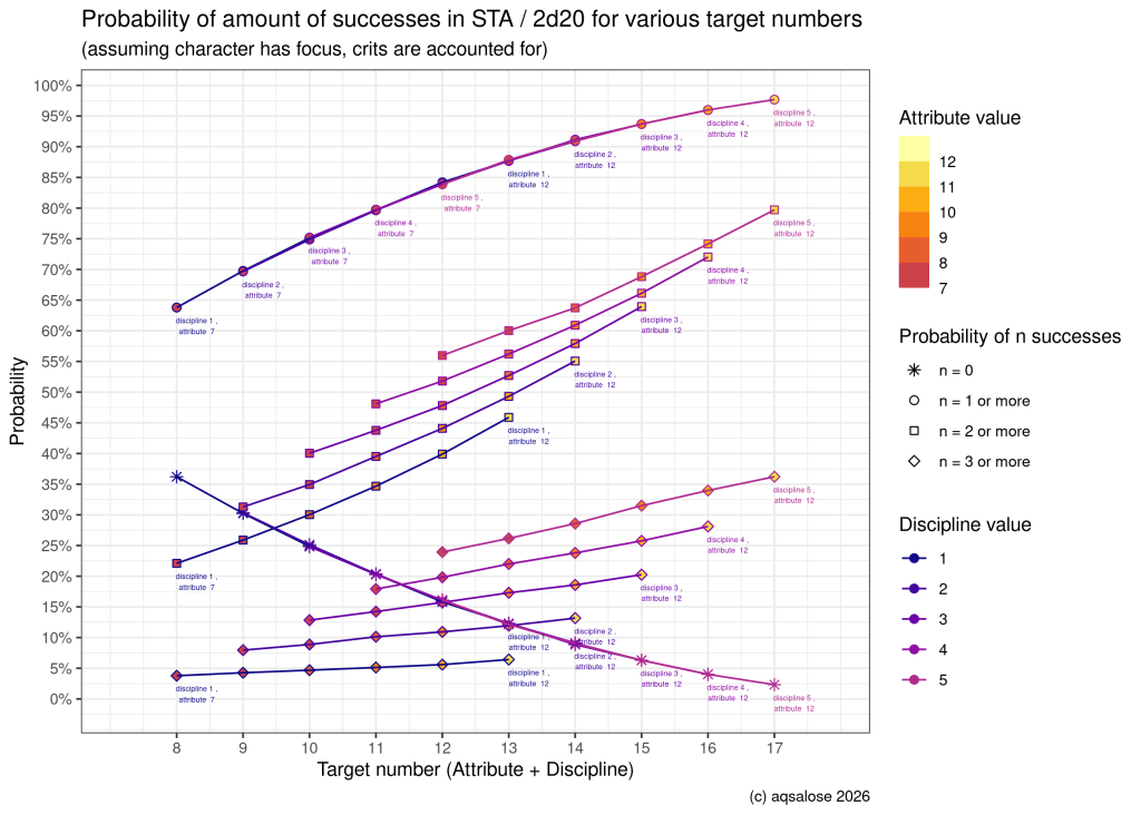
Here is the first figure, probability of 0 success, and 1 or more to 3 or more successes in 2d20, accounting for critical successes under focus.
In case that is hard to read, here is a plot where each difficulty (n successes) has its own faceted graph. I also had now more space to add n 4 and 5 (where 5 obviously is 0 when rolling 2 dice without assistance, but it’s useful later when we add comparisons with Momentum spends).
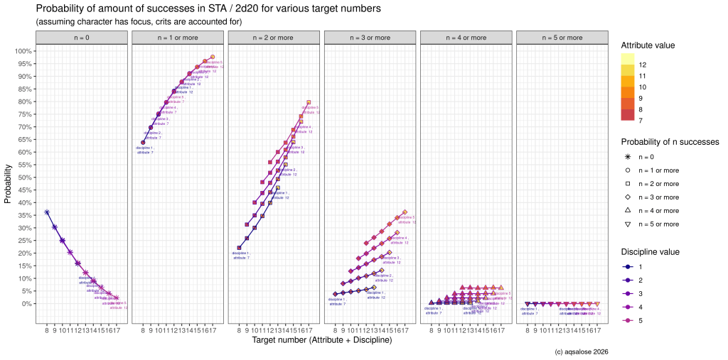
Technical digression: I don’t know if this style of plot has a name: initially I started by calculating the results and simply plotting probability of each one as a point, where on X-axis you have target number (attribute + discipline value sum) and on Y-axis the probability of the result. Because that was difficult to read, I added some shapes and colors and connecting lines.

Shapes denote number of successes (in practice, difficulty levels: 2 or more is needed to succeed at difficulty 2 tasks, and so on). Interior color denotes attribute value and outer color discipline value. (Different combinations of attribute and discipline values can yield same target number, but with a focus, different combinations have different probabilities to crit despite same target number.) Decision to connect same “discipline levels” rather than “attribute levels” is arbitrary, except for producing prettier result as color of both shapes and lines connecting them match (after I chose Discipline rather than Attribute as outer color).

Results are inexact from simulation, which causes small jitter.

Commentary

I don’t know if there is anything too surprising about any of this to experienced 2d20 players: it is commonly known that higher discipline + focus is more valuable than an attribute increase. I was slightly surprised by the exact scale of the crit benefit. At target number 12, low attribute but high discipline (A7+D5 and A8+D4) carry you to 50+% probability of success territory at difficulty 2. A11+D1 is approx 15 percentage points less valuable than A7+D5, “despite” same target number. It’s not that much, but succeeding slightly more often than failing rather failing slightly more often than succeeding is one of those things that intuitively feel like a lot in an extended campaign.

Looking it other way, if you started with combination of A7+D1 in some task of importance (success probability approx 23%), and you wanted (for some reason) increase that particular task performance in your next level-ups (milestones), you might consider while to using your milestones for one focus and 4 discipline increases, bringing you to A7+D5=12 and approx 55% success probability, rather than get 5 attribute increases, bringing you to A12+D1=13 and approx 46% success probability.

Impromptu journal club: Sander Greenland and P-values behaving exactly as they should

For the past year, the blog has been on an unscheduled hiatus because I felt I have very little to say. But this afternoon I stumbled upon a good article by Sander Greenland from 2018 [1] which “rehabilitates” P-values somewhat in my eyes.

Yes, I have used them in my work, but always felt a bit icky about it. Part of it is that during my undergraduate I found the Bayesian version of probability theory easier to reason about, and the Bayesians often scoff at frequentists. But the reasons to do so are real: Misinterpretations of p are common and easy (often I suspect I can’t keep the definitions exactly straight in my head); p is not the probability the alternative hypothesis is true; do I even know the null makes sense; the magical 0.05 boundary feels often both too small and too large and always unjustified; …. often, I have felt like writing verbal equivalents of bright yellow warning signs “I report a P-value because I think everyone wants it or everyone relevant already told me they want it; but you should be careful with it!!”

DANGER, WILL ROBINSON! P-VALUES! DANGER!

Greenland’s article was helpful to me because it clarifies both the misunderstandings of P-values and the way they should be correctly used from the point of view of someone who clearly wants to continue using them in stead of puffing some wild new framework like Bayes factors (okay he proposes S-values, but they are well-dressed P-values. I believe nobody will ever pick up Bayes factors.) The article manages to be clear about what you should do, in a way the statistics classes I had in school didn’t.

(The professors were clearly cognizant of the issues with P-values. I think I could still unearth old lecture notes with warnings to the effect “P-value is a probability of seeing the data under null, not the probability of null” and so on. But most often, the way people approach such message is by nodding sagely, and then proceed to report p and if it happens that p < 0.05, act like the null isn’t true.)

I found the article so helpful that I wanted to write it all down, in my own words (mostly). Each salient point has got its subheading, more or less in the same order as in the article [1].

Definitions are important

P-value, alpha, and p

Fisher’s definition: a P-value is the (tail) probability p under H that a test statistic would be as large or larger than what was observed, given the model A.

Neyman-Pearson definition: p is the smallest alpha level to allow rejection in an alpha-level Neyman-Person hypothesis test, rejecting H when p less or equal to alpha.

Neyman-Pearson is a mouthful to say, they are equivalent in all mathematical and computational senses. The difference is that in Neyman-Pearson framework, there is a fixed alpha-level. Alpha-level is fixed prior to seeing data and tells nothing of the data.

According to Greenland, P-value with capital P often refers to the random variate P. Small letter p refers to the observed P-value which is data and sample dependent numerical quantity, like often X is a random variable and x an instance of it. Yet not everyone is aware of other statisticians making this distinction. This causes confusion.

Significance level

Fisher used significance level as synonymous to p. Many other use it and refer to alpha. This causes confusion.

Compatibility, not error probability

The P-value is can be understood as function of data that describes compatibility of observed sample with the (null) hypothesis H (given model A). I agree this presentation is good, because it makes it explicit that there could be other hypothesis H’ (other model A’) with similar observed “compatibility”.

Relatedly, Greenland argues the P-value is often misunderstood if defined as Type I error probability (probability of rejecting H when H is true). While it is true theoretically, it may not be true in practice. On the hand, it makes it easy to confuse p with alpha; alpha is the specified intended Type I error bound. Quote:

The actual Type-I error rate of a test of the hypothesis H given the assumptions A is often unknown to the investigator, because it may deviate from α due to defects in A or discreteness of the data. 4 In contrast, α is defined as the maximum tolerable Type-I error rate, which is set by the investigator and thus is known; p is then compared to this α to make decisions, on the assumption that the corresponding random P is valid (which makes α equal to the Type-I error rate).

S. Greenland, [1]

Alpha level should depend on the cost of rejection

It is very common just pick alpha level 0.05. Greenland mentions this point only in passing, but I think it is an important one. For different purposes different alpha is needed, because the cost of wrong decision may be context dependent. This is also a good reason to present an unadjusted p-value.

I only wish the process of determining the true cost of false positives were given more thought in general and statistics education.

Not only nulls

You may have noticed already there has not been much talk of “null” hypothesis written as H0 yet. Greenland thinks calling H null was an unfortunate mistake by Fisher, further confused by some ways to read Neyman-Pearson decision theory. This leads to confusion as some people think that only null hypotheses of no effect can / should be tested.

The P-value should be best thought in relation a tested hypothesis H, true. But P-value could and should be computed for many hypothesized effects, not only “no effect”. Especially if prior to study one has a guess of the effect, maybe even has computed a power analysis with this effect, one should compute P-value for this effect.

(Comment: For point hypothesis and point estimates, this aspect is visually alleviated by showing the confidence intervals. But confidence intervals are not panacea. For instance, 95% CI is restricted to 95% and often the best you can say looking at them is that p for a given effect is either < 0.05 or > 0.05.)

P-values do not measure population parameter and are not expected to converge

One common complaint against P-values Greenland disagrees with is the disappointment that P-values are random. The argument is as follows:

By definition, if the tested hypothesis H is true (and model A holds), P-values should be distributed uniformly randomly. (After all, their whole computation is intimately tied to this property.) They are not a population parameter, they describe the variation of the estimated effect b (given H and A). Nobody should be aghast if the P-values from previous studies are not replicated in a new study.

However, Greenland also points out that if distribution of P is not uniform under replicated sampling, it is an indication that either H or A is wrong.

On this point, I disagree with Greenland’s framing: I think most people understand that P are distributed and assumed uniform under null, and do not expect converging P in replications. I believe they expect to see some very starkly non-uniform distribution (in form of more small p). This is because people understandably wish to see small p in their replication because they have read a publication that told there is some effect, significant at p<0.05, and expect that if there is true effect, their replication would also yield a small P-value.

(van Zwet and Goodman have recent interesting paper about how large study one should conduct to have high enough power to warrant expectations of a successful replication [2])

And finally, G. well points out one should remember that if distribution of P is uniform, it doesn’t prove H and A are correct. It is possible the test simply doesn’t reflect the part where A and H fail.

P-values relate effect size to sample size

What it says in the subtitle above. I have always found this easy to understand, but apparently some people have lamented that “P-values confound effect size with sample size”. I found this information surprising.

S-value

Recall an earlier paragraph where the P-value was defined as a measure of compatibility. Unfortunately it is a poor measure of compatibility; here I found it easiest to simply quote Greenland:

The scaling of p as a measure is poor, however, in that the difference between (say) 0.01 and 0.10 is quite a bit larger geometrically than the difference between 0.90 and 0.99. For example, using a test statistic that is normal with mean zero and standard deviation (SD) of 1 under H and A, a p of 0.01 vs. 0.10 corresponds to about a 1 SD difference in the statistic, whereas a p of 0.90 vs. 0.99 corresponds to about a 0.1 SD difference.

S. Greenland, [1]

Greenland suggests using S-value instead, where S stands for Shannon, and defined as

s=  - \log_2 p  \quad (= \log 1/p).

It can be interpreted as self-information or surprisal, measured in bits.

P-values do not overstate evidence, people don’t understand p-values

…and S-values are supposed to help with this.

Here the argument is that people overestimate badly how (un)likely p <0.05 is by fixating on 0.05 and thinking it is “significant”. By using the S-value, one sees that p = 0.05 corresponds only about 4 bits of information against a hypothesis, not much more.

What it means to have 4 bits of evidence / information? Here I again found it easiest to quote:

To provide an intuitive interpretation of the information conveyed by s, let k be the nearest integer to s. We may then say that p conveys roughly the same information or evidence against the tested hypothesis H given A as seeing all heads in k independent tosses of a coin conveys against the hypothesis that the tosses are “fair” (each independent with chance of heads =1/2) versus loaded for heads; k indicator variables all equal to 1 would be needed to represent this event.

ibid [1]

P values are sensitive to sample size, which should be accounted by refining hypothesis

No, you have not made error scrolling. There was a previous point about P-values conflating effect sizes with sample sizes. However, ignoring the effect, P-values have a habit of getting very small with very large data “on their own”. Small P-value is a sign that either hypothesis H or the model A is wrong; because most models are at least somewhat wrong (remember how statisticians like to quote George Box, “all models are wrong but some are useful”), with enough samples the imprecision – but not the kind that one expects – can result in a small P-value.

Greenberg notes that this critique describes a true phenomenon that happens, but should not be held against P-value: P-value is doing its job correctly showing in a large enough data that the model you thought useful is not correct one. What Greenland says you should do, is to think more about your hypothesis.

The solution proposed is to use interval hypothesis instead of testing a point estimate hypothesis. P-values are equally valid for interval (or region) hypotheses as point hypotheses; it is researcher’s, not P-values fault the researcher choses a bad hypothesis.

I think interval hypotheses are also good, but slightly other reason: instead of testing whether the effect is exactly zero it is a good idea to think about what effect would be practically zero. I am less convinced about relation to sample size sensitivity. (Now I want to run some simulations to get a good practical grip on when model misspecification or close-to-point-hypothesis effect result in small p-values.)

Large p is not a safety signal

This is a point worth hammering down, even though I think it was already said many times. Greenland also presents another S-value argument. Remember that 95% CI corresponds to S-value of 4.3 bits, which was an argument for 0.05 being an unimpressive p? Another interpretation of the same CI is that any point within 95% CI of an estimate has only max 4.3 bits of “refutational information” against it. In other words, you can’t well rule out anything inside CI.

The paper quotes a good example of a mistake: study estimated 95% CI that covered RR from 2/3 to 5, which was summarized to the effect ” relative risk not significantly different from 1″. Yet notice that CI included anything from 1 to 5 fold relative risks! G. correctly notes that the true conclusion is that study was so small that there was good enough information to rule out only very extreme RRs.

My conclusions, bit different from the author’s

So, I said the article rehabilitated P-value in my eyes. The reason is that it outlines many of the issues of P-value and provides solutions:

  1. Do not overly focus on traditional alpha values, try to think what alpha makes sense for your application. (This BTW also applies to CI.)
  2. Do not blindly trust p is a type I error rate.
  3. If you find it helpful, you could think in terms of S-values and bits of information.
  4. Test all relevant hypotheses. Consider also your model and sample size. Sometimes the relevant hypothesis is a region or an interval.

The author’s conclusions can be found by reading the paper.

References

[1] Greenland, Sander. “Valid P-Values Behave Exactly as They Should: Some Misleading Criticisms of P-Values and Their Resolution With S-Values.” The American Statistician 73, no. sup1 (March 29, 2019): 106–14. https://doi.org/10.1080/00031305.2018.1529625. https://www.tandfonline.com/doi/full/10.1080/00031305.2018.1529625 (openly accessible)

[2] Zwet, Erik W. van, and Steven N. Goodman. “How Large Should the next Study Be? Predictive Power and Sample Size Requirements for Replication Studies.” Statistics in Medicine 41, no. 16 (2022): 3090–3101. https://doi.org/10.1002/sim.9406. https://onlinelibrary.wiley.com/doi/full/10.1002/sim.9406

How to export your GoodReads data as CSV

Summary in Finnish: Amazonin lukupäiväkirja-arkiston käyttäjä esittää kuva-arvoituksen varmuuskopiointia varten.

Introductory musings

It is a curious time to come back to blogging! People (re-)launch blogs here and there, except they are being luddites about it: they are turning back to old tried and tested technology solutions, that is, running email newsletters (to great surprise of everyone)! I, for one, feel like a modern person for deciding to buy me some WordPress-as-a-service.

In all seriousness, I have been writing two (quite unfinished) long post drafts to properly celebrate the Grand Blog Re-Opening. However, recently I heard someone to point out that one can export ones GoodReads library as a CSV, and today while updating my reading lists, I decided to try and find the relevant UI menu to point and click. Turns out, the relevant button is not exactly hidden but not as easy to find than as I thought either, and as I doubt not too many people are aware of this useful feature (I wasn’t!), I thought it would be worth someone’s while to document the procedure. (As an additional plus, this write-up is quick and simple compared to the other aforementioned drafts I am working on.)

So is the feature useful? Based on cursory checks, the CSV output is reasonably well-constructed (with commas as separators) and easily digested by LibreOffice parser. It contains GR book id, title, author information, your and users’ average rating, publishing information, date added (in US format, urgh), your bookshelves it is in (if you have any), and your review (if you did write one). I evaluate it looks quite useful for making backups! (Why backups? Maybe one day Amazon won’t find any utility from GR and turns it off, or will turn evil and use it for uncouth purposes! It is a good principle try to be your own master in matters concerning your data: I am glad I can say for once I am favorably surprised by a social media service.)

The tutorial

My first guess was to look in the Settings menu. It is not there! Instead:

  1. Navigate to My Books.

2. Good! Scroll down.

3. Locate the Import and export button.

4. Click the thing there, wait a moment, and you are ready.

5. Inspect the downloaded CSV at your leisure.

Yes, I know there are “better” tools than LibreOffice Calc, but (a) it has a GUI (b) it works reasonably well when you double-click the file in Nautilus in Ubuntu.

That’s all this time. Next time I’ll have something more highbrow.

Example Lorem Ipsum no 2: Electric Boogaloo

This is an another example placeholder post. I am using it to test category-based filters in the widgets on the main page! It will be replaced with actual content soon! Meanwhile, enjoy more of ol’ good classic Lorem Ipsum.

“Electric Boogaloo”? Let TvTropes explain it all here.

Lorem ipsum dolor sit amet, consectetur adipiscing elit, sed do eiusmod tempor incididunt ut labore et dolore magna aliqua. Ut enim ad minim veniam, quis nostrud exercitation ullamco laboris nisi ut aliquip ex ea commodo consequat. Duis aute irure dolor in reprehenderit in voluptate velit esse cillum dolore eu fugiat nulla pariatur. Excepteur sint occaecat cupidatat non proident, sunt in culpa qui officia deserunt mollit anim id est laborum.

Et harum quidem rerum facilis est et expedita distinctio. Nam libero tempore, cum soluta nobis est eligendi optio, cumque nihil impedit, quo minus id, quod maxime placeat, facere possimus, omnis voluptas assumenda est, omnis dolor repellendus. Temporibus autem quibusdam et aut officiis debitis aut rerum necessitatibus saepe eveniet, ut et voluptates repudiandae sint et molestiae non recusandae. Itaque earum rerum hic tenetur a sapiente delectus, ut aut reiciendis voluptatibus maiores alias consequatur aut perferendis doloribus asperiores repellat…